

An Illustrative Model of Housing Prices
An Illustrative Model of Housing Prices
Taking into account regional income differences can help us understand the behavior of housing markets.

Thank you for reading our work! If you haven’t yet subscribed, please subscribe below:
If you would like to support us further with reaching our 1,000 subscriber goal by year end, please consider sharing and liking this article!
As Nominal News grows larger, we will be able to make this a full-time project, and provide more content. If you would like to suggest a topic for us to cover, please leave it in the comment section.

Several weeks ago, we completed a holistic multi-part overview on the issues of house prices and housing affordability:
The focus of those articles is on the research regarding house price determination and how prices respond to policy changes. The key findings of the research we reviewed can be summarized as follows:
House prices are significantly above replacement cost in approximately 15% of US metropolitan areas (data from 2013);
In most areas, house prices are less than 125% of replacement cost (data from 2013);
These elevated house prices occur in areas where incomes are high and there is no excess housing available and limited developable vacant land;
The spend on housing and transportation together as a share of income across cities is quite similar;
House prices, in urban areas, appear to respond very little to large increases in upzoning and housing stock increases (for example, a 36% upzoning in Sao Paulo, which lead to a 2% increase in housing stock, reduced prices by 0.5%);
During the Covid pandemic, rents significantly dropped in many of the high cost urban areas.
Let’s go over the intuition which can effectively capture all these findings of the housing market with some visual aids we made thanks to Canva.
The Model
A House
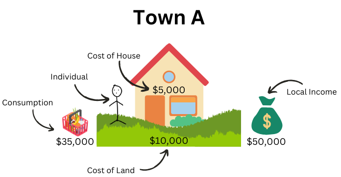
A house (or apartment) allows an individual to live in the particular area. By living in the area, the individual can earn a particular local income. To live in that particular area, the individual has to pay for the house (predominantly construction costs) and the land (value of living in the area). Assume that these costs are annual flows (as if paying rent to a landlord). After these costs, the individual spends the rest on a basket of consumption goods, such as food, clothing, entertainment, etc. (we are simplifying this issue by ignoring things like savings, taxes, etc). In our example above, the individual earns $50,000 and spends $15,000 on the house, leaving $35,000 for the individual per year to spend on consumption..
Adding a New Town
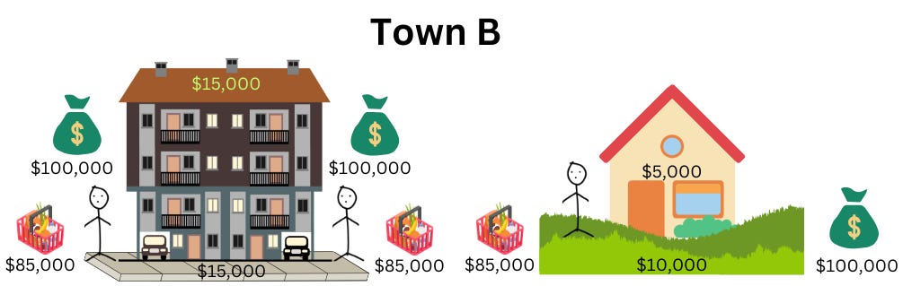
Now suppose there is a Town B, not far from Town A:
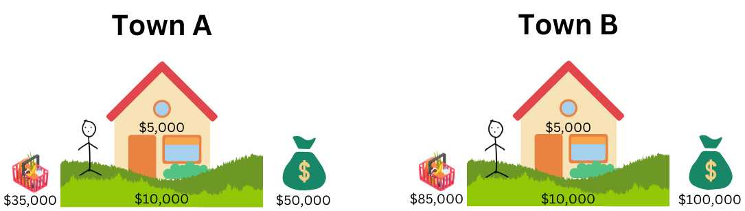
In Town B, an Individual B that is more or less identical to our previous individual A (same skill level, age, profession, etc.), earns $100,000. If we assume that land and building materials are abundant, Individual B will also spend $15,000 on housing and thus have $85,000 leftover for consumption.
The reason why Town B might offer higher income for the same worker is because Town B may have more productive firms with better technologies and machines. Thus, the worker can be more productive in the firm in Town B than in Town A, and receives higher compensation.
Allowing Movement
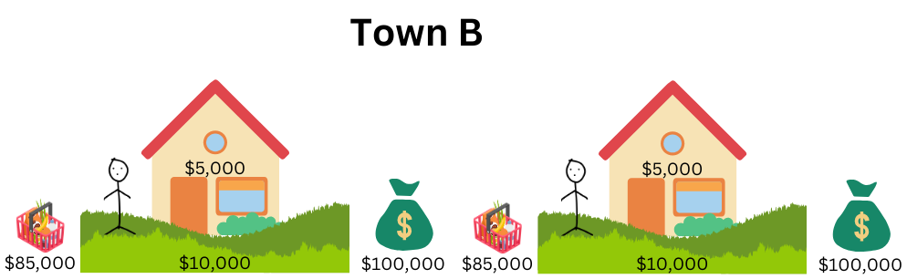
Suppose now we allow each individual to choose where to live. Let’s also simplify the scenario and abstract away from any moving costs (normally, moving from one town to another should entail some costs). If you’re Individual A, you note that you would be much better off in Town B since you will have $85,000 remaining for consumption, which is $50,000 more than you have in Town A. Individual A would then want to move to Town B. If Town B has available land, they will just buy the land and build a house:
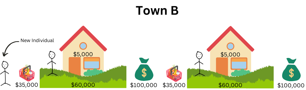
Suppose another individual from Town A wants to move to Town B:

If there’s no more space to build and no construction ability, the new individual would need to bid on the house. What would be their maximal willingness to pay for this house? Well, in Town A they had $35,000 of consumption, so as long as they made that amount, they would choose to move to Town B. Thus, they would bid up the house all the way to $65,000. Since the physical structure is just $5,000, the land would now be worth $60,000.
It is worth noting a few additional things. The new third individual from Town A was only making $35,000 (after expenses) and thus might not be able to pay the $65,000 for the house in Town B. This is where we assume mortgage financing is ‘perfect’. That is, a bank offering the mortgage would permit taking out a large mortgage and also accept that the individual will be making the $100,000 and thus, would be able to make the $65,000 payment. This is how future incomes play a key role in determining house prices. If we were to assume that financing isn’t ‘perfect’ (banks are hesitant to give such loans), then the price would be below $65,000, as it would be restricted by how much the bank is willing to offer as a mortgage.
This is where mortgage subsidies (via the 30 year mortgage) can impact house prices. By providing such a subsidy, banks are willing to offer higher mortgages, and thus individuals are able to pay more for the same house, bringing back the price close to its maximum (i.e. $65,000).
Densification
Suppose now that in Town B, one of the plots of land is densified, and instead of one house, two apartments that are identical to the house can be built (we are assuming this for simplicity). Let’s also assume that densifying is costlier – that is, two identical houses on one plot of land have a higher total construction cost than building two separate houses on two plots of land. If we just have 3 people, we will now have 3 houses and satisfy the demand for living in Town B.
In our case, we assume the left structure costs $15,000 to build (more than two times $5,000). So what would be the price of land then? Well, if it remained $10,000, each individual in the upzoned area would make $100,000 - $7,500 (half construction cost) - $5,000 (half land cost) = $87,500. That means the individual in the single home would be worse off since they are making only $85,000. They would immediately want to move into the upzoned apartment, and thus bid up the price, from $10,000 to $15,000, until they would be indifferent. Thus, the land price would need to be $15,000, since then, each individual in the upzoned apartments makes $85,000. Each dwelling still costs $15,000 to each individual in Town B.
It’s worth noting that in real life, the individual living in the single house might be perfectly happy paying a higher fraction of their income to live in a not-densified area. Then, the consumption basket differential of $87,500 and $85,000 could be sustainable, as there is an amenity value of $2,500 to the single home occupier. However, for now, we are abstracting away from amenity values.
Another Individual and Further Upzoning
Now suppose there is another individual from Town A wanting to move to Town B. Similarly, if there is insufficient housing, the prices of all houses in Town B would be bid up until everyone makes $35,000 in consumption. This would imply that the two apartments together would cost $130,000 ($15,000 construction cost, $115,000 land value), leaving each individual with 35k in consumption income.
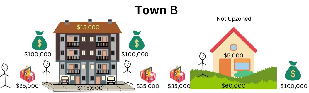
What if we were to upzone the other parcel of land and allow for two homes on it as well, but chose not to build on this parcel of land?
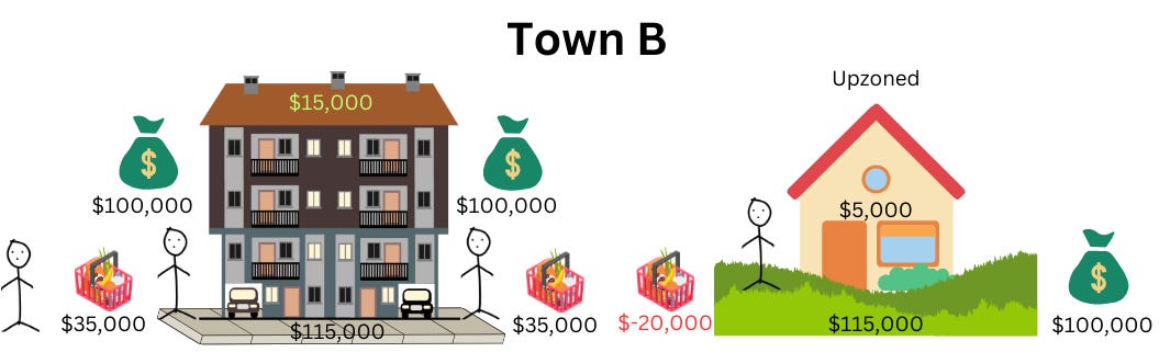
Since the landlord of the single family home would prefer to build the apartment complex, as they would get $115,000 for the land, instead of $60,000, the landlord would charge the higher price for that land. This means that the individual living in the single home would actually not be able to afford this home and thus would need to move out resulting in an apartment complex being built. Alternatively, a person with a higher income could move in, if they were to have an amenity value (or preference) for living in a single home.
The Long Run
In the above scenario, land prices increased in Town B because there were not enough houses for everyone wanting to live in Town B. If we did have sufficient housing to meet demand of all individuals, the price of an individual home would then simply reflect construction costs ($5,000) and universal land costs ($10,000), like in Town A in this model. So why are housing costs in cities (Town Bs) often significantly above construction costs? This is predominantly driven by the fact that there is a lot of demand to live in cities as the population of the US is large – there are basically a lot of Town A people. On the other hand, there are few Town Bs that offer very large incomes compared to Town As. A balance where Town B offers high income and has Town A housing prices simply cannot exist in equilibrium, as that would mean everyone would live in Town B.
Naturally, there are limiting factors to how many people can be located in Town B. These are often physical limitations – mainly available land, but also the transportation. Although we did not mention it in our model above, transportation is necessary for people to actually get the income in any town (commuting to work). As discussed in our previous article, it turns out that many of the ‘unaffordable’ cities are affordable once we take into account transportation since using the subway is much cheaper than driving. Nonetheless, even public transit can physically move a limited number of people. Cities most likely have a maximal population before congestion becomes too burdensome.
It appears, therefore, that high income cities will always have relatively more expensive housing. In Town A, you spent only 30% of income on housing, while in Town B the number was 65%. However, both citizens of Town A and Town B were just as happy in how much they consume (the same amount) so percentage spent on housing is not necessarily relevant.
Why Prices Still Fall When We Build
The above model suggests that, as long as there is enough demand (Town A people), prices would not move down in Town B even if we build additional housing. Now although research has shown that house prices are not that sensitive to new construction (and our model captures that), prices do fall when new construction occurs (for a 2% increase in housing stock, prices fall by 0.5%). In order to capture this fact, we would need to loosen our simplifying assumption that each individual is identical. In reality, we know people have preferences and may value non-income factors as well, such as simply preferring Town A because you were born there (in economics, we call these ‘taste preferences').
Thus, in a supply constrained market such as Town B, everyone who lives there must have the highest willingness to pay. Anyone who does not live there, must have a marginally lower willingness to pay for some reason, or else they would live in Town B, where they can make a higher income. Thus, an additional apartment built in Town B will be taken by someone that has a slightly lower willingness to pay than all current residents of Town B. But that implies a falling price of all units because the price would be determined by the person in Town B with the lowest willingness to pay.
Since additional housing has a marginal impact on pricing (2% increase in housing stock reduces prices by 0.5%), this suggests that many people living outside of high income urban areas have almost as high willingness to pay and preferences of living in these areas, as the people located there.
Additional Abstractions
In our model, we made a lot of simplifying assumptions. Many of these assumptions can be weakened, which would allow us to match reality better, but the underlying mechanisms regarding price behavior would remain. Here are a few examples of ‘weakening’ the assumptions:
Allowing city income to be uncertain would make urban living riskier as people cannot guarantee they will find a job – this would reduce urban land values in our model;
Taking into account that goods and services in cities are more expensive, meaning the consumption baskets between Town A and Town B are not comparable – this would reduce urban land values;
Taking into account the agglomeration effect, which tells us that if more people are in a particular area, all individuals are more productive, which would increase incomes – this increases urban land values;
Taxation of both incomes and land has significant impacts on the amount of take home pay – this would reduce urban land values.
If we were to incorporate all the extra elements, then the land prices observed in Town B would be less sensitive to housing prices and incomes in Town A since these other factors also influence the price in Town B. In our current simplified model, consumption baskets are equalized between Town A and Town B. Basically, land prices in Town B are such that the residual income of an individual Town B is equivalent to the residual income of an individual in Town A. However, if an individual in Town B takes on more risk (i.e. uncertain income), they’d expect to have a higher consumption basket on expectation as a reward for taking this risk.
Conclusion
After writing a three-part series on housing research, I wanted to put together all the key findings and what they imply. The above process is also how economic research ideas are often formulated:
Data and patterns are observed;
A model is designed that can capture some of these patterns;
The model is then tested with the data to see whether it captures these and other fact patterns (which we did not perform here);
Policy experiments can be run on the model.
Overall, it appears that as long as income is tied to land and location, increasing the amount of money people have after paying for housing (i.e. improving affordability) will be difficult. Certainly, building more houses in cities is still a benefit, as it allows more people to be in a productive area, but unless we observe extremely large supply increases, prices will remain relatively stable. On the other hand, the COVID pandemic showed us how urban house prices and rents collapsed when incomes were decoupled from locations.
Interesting Reads from the Week
News: The most recent Consumer Price Index (CPI) came in ‘high’ for February at 0.4% month-over-month. However, as discussed previously at Nominal News, a lot of this is driven by past housing inflation given how shelter inflation is accounted for.
- tackles the latest jobs market data and what it implies about the current state of the economy.
- and discuss the recent large jump in poverty in the US, and how what a Universal Basic Income (UBI) study in Kenya can tells us about tackling this problem.
Photo by Pok Rie.
If you enjoyed this article, you may also enjoy the following ones from Nominal News:
Monopolies and Antitrust Enforcement (November 20, 2023) – with news of the Federal Trade Commission suing Amazon for anti-competitive practices, economic research suggests that such lawsuits typically improve overall welfare.
To Compete or Non-Compete (April 30, 2023) – why non-compete clauses do not solve any issues, but only create costs.
Discrimination in Real Estate (September 17, 2023) – unlike explicit discrimination, statistical discrimination is less talked about. However, it has significant impacts on outcomes for people impacted by it. Real estate agents, often unaware of their own statistical discrimination, end up perpetuating outcomes for minorities.
Very nice piece explaining housing prices with some simple, easy to understand, models. I like it.
Generally speaking, as I will explore in an upcoming essay in Risk & Progress, we want our cities to be big. Scaling laws show super linear outputs (GDP, incomes, patent applications…etc) as the population grows with sublinear inputs (highways, phone lines, electric lines…etc).